OpenCV3的机器学习算法SVM-使用Python
Goal
In this chapter
We will see an intuitive understanding of SVM
目标
• 对 SVM 有一个直观理解
Theory
Linearly Separable Data
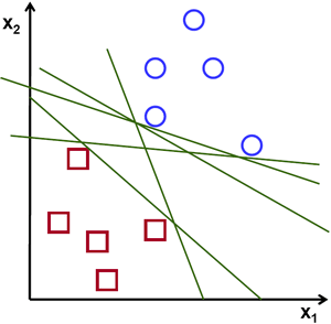
Consider the image below which has two types of data, red and blue. In kNN, for a test data, we used to measure its distance to all the training samples and take the one with minimum distance. It takes plenty of time to measure all the distances and plenty of memory to store all the training-samples. But considering the data given in image, should we need that much?
原理线性数据分割
如下图所示,其中含有两类数据,红的和蓝的。如果是使用 kNN,对于一 个测试数据我们要测量它到每一个样本的距离,从而根据最近邻居分类。测量 所有的距离需要足够的时间,并且需要大量的内存存储训练样本。但是分类下 图所示的数据真的需要占用这么多资源吗?

image
Consider another idea. We find a line, f(x)=ax1+bx2+c which divides both the data to two regions. When we get a new test_data X, just substitute it in f(x). If f(X)>0, it belongs to blue group, else it belongs to red group. We can call this line as Decision Boundary. It is very simple and memory-efficient. Such data which can be divided into two with a straight line (or hyperplanes in higher dimensions) is called Linear Separable.
我们在考虑另外一个想法。我们找到了一条直线,f (x) = ax1 + bx2 + c, 它可以将所有的数据分割到两个区域。当我们拿到一个测试数据 X 时,我们只 需要把它代入 f (x)。如果 |f (X)| > 0,它就属于蓝色组,否则就属于红色组。 我们把这条线称为决定边界(Decision_Boundary)。很简单而且内存使用 效率也很高。这种使用一条直线(或者是高位空间种的超平面)上述数据分成 两组的方法成为线性分割。
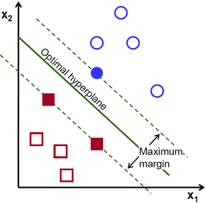
So in above image, you can see plenty of such lines are possible. Which one we will take? Very intuitively we can say that the line should be passing as far as possible from all the points. Why? Because there can be noise in the incoming data. This data should not affect the classification accuracy. So taking a farthest line will provide more immunity against noise. So what SVM does is to find a straight line (or hyperplane) with largest minimum distance to the training samples. See the bold line in below image passing through the center.
从上图中我们看到有很多条直线可以将数据分为蓝红两组,那一条直线是 最好的呢?直觉上讲这条直线应该是与两组数据的距离越远越好。为什么呢? 因为测试数据可能有噪音影响(真实数据 + 噪声)。这些数据不应该影响分类 的准确性。所以这条距离远的直线抗噪声能力也就最强。所以 SVM 要做就是 找到一条直线,并使这条直线到(训练样本)各组数据的最短距离最大。下图 中加粗的直线经过中心。

image
So to find this Decision Boundary, you need training data. Do you need all? NO. Just the ones which are close to the opposite group are sufficient. In our image, they are the one blue filled circle and two red filled squares. We can call them Support Vectors and the lines passing through them are called Support Planes. They are adequate for finding our decision boundary. We need not worry about all the data. It helps in data reduction.
要找到决定边界,就需要使用训练数据。我们需要所有的训练数据吗?不, 只需要那些靠近边界的数据,如上图中一个蓝色的圆盘和两个红色的方块。我 们叫他们支持向量,经过他们的直线叫做支持平面。有了这些数据就足以找到 决定边界了。我们担心所有的数据。这对于数据简化有帮助。
What happened is, first two hyperplanes are found which best represents the data. For eg, blue data is represented by wTx+b0>1 while red data is represented by wTx+b0<−1 where w is weight vector ( w=[w1,w2,...,wn]) and x is the feature vector ( x=[x1,x2,...,xn]). b0 is the bias. Weight vector decides the orientation of decision boundary while bias point decides its location. Now decision boundary is defined to be midway between these hyperplanes, so expressed as wTx+b0=0. The minimum distance from support vector to the decision boundary is given by, distancesupportvectors=1||w||. Margin is twice this distance, and we need to maximize this margin. i.e. we need to minimize a new function L(w,b0) with some constraints which can expressed below:
minw,b0L(w,b0)=12||w||2subject toti(wTx+b0)≥1∀i
where ti is the label of each class, ti∈[−1,1]
.
到底发生了什么呢?首先我们找到了分别代表两组数据的超平面。例如,蓝 色数据可以用 ωT x+b0 > 1 表示,而红色数据可以用 ωT x+b0 < −1 表示,ω 叫 做权重向量(ω = [ω1,ω2,...,ω3]),x 为特征向量(x = [x1,x2,...,xn])。b0 被
成为 bias(截距?)。权重向量决定了决定边界的走向,而 bias 点决定了它(决
定边界)的位置。决定边界被定义为这两个超平面的中间线(平面),表达式为
ωT x+b0 = 0。从支持向量到决定边界的最短距离为 distancesupport vector = 1 。||ω||
边缘长度为这个距离的两倍,我们需要使这个边缘长度最大。我们要创建一个 新的函数 L (ω, b0) 并使它的值最小:
其中 ti 是每一组的标记,ti ∈ [−1, 1]。
Non-Linearly Separable Data
Consider some data which can't be divided into two with a straight line. For example, consider an one-dimensional data where 'X' is at -3 & +3 and 'O' is at -1 & +1. Clearly it is not linearly separable. But there are methods to solve these kinds of problems. If we can map this data set with a function, f(x)=x2, we get 'X' at 9 and 'O' at 1 which are linear separable.
非线性数据分割
想象一下,如果一组数据不能被一条直线分为两组怎么办?例如,在一维 空间中 X 类包含的数据点有(-3,3),O 类包含的数据点有(-1,1)。很明显 不可能使用线性分割将 X 和 O 分开。但是有一个方法可以帮我们解决这个问 题。使用函数 f(x) = x2 对这组数据进行映射,得到的 X 为 9,O 为 1,这时 就可以使用线性分割了。
Otherwise we can convert this one-dimensional to two-dimensional data. We can use f(x)=(x,x2) function to map this data. Then 'X' becomes (-3,9) and (3,9) while 'O' becomes (-1,1) and (1,1). This is also linear separable. In short, chance is more for a non-linear separable data in lower-dimensional space to become linear separable in higher-dimensional space.
或者我们也可以把一维数据转换成两维数据。我们可以使用函数 f (x) =(x, x2 ) 对数据进行映射。这样 X 就变成了(-3,9)和(3,9)而 O 就变成了 (-1,1)和(1,1)。同样可以线性分割,简单来说就是在低维空间不能线性分割的数据在高维空间很有可能可以线性分割。
In general, it is possible to map points in a d-dimensional space to some D-dimensional space (D>d) to check the possibility of linear separability. There is an idea which helps to compute the dot product in the high-dimensional (kernel) space by performing computations in the low-dimensional input (feature) space. We can illustrate with following example.
通常我们可以将 d 维数据映射到 D 维数据来检测是否可以线性分割(D>d)。这种想法可以帮助我们通过对低维输入(特征)空间的计算来获得高 维空间的点积。我们可以用下面的例子说明。
Consider two points in two-dimensional space, p=(p1,p2) and q=(q1,q2). Let ϕ be a mapping function which maps a two-dimensional point to three-dimensional space as follows:
ϕ(p)=(p21,p22,2‾√p1p2)ϕ(q)=(q21,q22,2‾√q1q2)
Let us define a kernel function K(p,q) which does a dot product between two points, shown below:
K(p,q)=ϕ(p).ϕ(q)ϕ(p).ϕ(q)=ϕ(p)Tϕ(q)=(p21,p22,2‾√p1p2).(q21,q22,2‾√q1q2)=p1q1+p2q2+2p1q1p2q2=(p1q1+p2q2)2=(p.q)2
假设我们有二维空间的两个点:p = (p1, p2) 和 q = (q1, q2)。用 Ø 表示映 射函数,它可以按如下方式将二维的点映射到三维空间中:
我们要定义一个核函数 K (p, q),它可以用来计算两个点的内积,如下所示
It means, a dot product in three-dimensional space can be achieved using squared dot product in two-dimensional space. This can be applied to higher dimensional space. So we can calculate higher dimensional features from lower dimensions itself. Once we map them, we get a higher dimensional space.
这说明三维空间中的内积可以通过计算二维空间中内积的平方来获得。这 可以扩展到更高维的空间。所以根据低维的数据来计算它们的高维特征。在进 行完映射后,我们就得到了一个高维空间数据。
In addition to all these concepts, there comes the problem of misclassification. So just finding decision boundary with maximum margin is not sufficient. We need to consider the problem of misclassification errors also. Sometimes, it may be possible to find a decision boundary with less margin, but with reduced misclassification. Anyway we need to modify our model such that it should find decision boundary with maximum margin, but with less misclassification. The minimization criteria is modified as:
min||w||2+C(distanceofmisclassifiedsamplestotheircorrectregions)
除了上面的这些概念之外,还有一个问题需要解决,那就是分类错误。仅 仅找到具有最大边缘的决定边界是不够的。我们还需要考虑错误分类带来的误 差。有时我们找到的决定边界的边缘可能不是最大的但是错误分类是最少的。 所以我们需要对我们的模型进行修正来找到一个更好的决定边界:最大的边缘, 最小的错误分类。评判标准就被修改为:
Below image shows this concept. For each sample of the training data a new parameter ξi is defined. It is the distance from its corresponding training sample to their correct decision region. For those who are not misclassified, they fall on their corresponding support planes, so their distance is zero.
下图显示这个概念。对于训练数据的每一个样本又增加了一个参数 ξi。它 表示训练样本到他们所属类(实际所属类)的超平面的距离。对于那些分类正 确的样本这个参数为 0,因为它们会落在它们的支持平面上。

image
So the new optimization problem is :
minw,b0L(w,b0)=||w||2+C∑iξi subject to yi(wTxi+b0)≥1−ξi and ξi≥0 ∀i
How should the parameter C be chosen? It is obvious that the answer to this question depends on how the training data is distributed. Although there is no general answer, it is useful to take into account these rules:
Large values of C give solutions with less misclassification errors but a smaller margin. Consider that in this case it is expensive to make misclassification errors. Since the aim of the optimization is to minimize the argument, few misclassifications errors are allowed.
Small values of C give solutions with bigger margin and more classification errors. In this case the minimization does not consider that much the term of the sum so it focuses more on finding a hyperplane with big margin.
现在新的最优化问题就变成了:
参数 C 的取值应该如何选择呢?很明显应该取决于你的训练数据。虽然没 有一个统一的答案,但是在选取 C 的取值时我们还是应该考虑一下下面的规 则:
如果 C 的取值比较大,错误分类会减少,但是边缘也会减小。其实就是 错误分类的代价比较高,惩罚比较大。(在数据噪声很小时我们可以选取 较大的 C 值。)
如果 C 的取值比较小,边缘会比较大,但错误分类的数量会升高。其实 就是错误分类的代价比较低,惩罚很小。整个优化过程就是为了找到一个 具有最大边缘的超平面对数据进行分类。(如果数据噪声比较大时,应该 考虑)
Additional Resources
.